In the last few days there has been a discussion about VLookup and how the last parameter works when it is entered as TRUE, FALSE or omitted altogether.

The Microsoft Help page was showing an example screenshot, where the formula and the result did not match up.

This was an oversight in the help documentation and will be fixed.

But it sparked a few questions, like:

• Why do I get an error for this formula, but when I expand the lookup table by one row I get the correct result?
  

With the last parameter set to 0 or FALSE, Vlookup will go through the list from the top, one cell after the other, and will compare each value in the first column to the lookup value. The list does not need to be sorted. When it finds a match, it returns the value from the specified column. For large lists, this can be rather slow.

Vlookup with the 1 or TRUE as the last parameter (omitting the parameter defaults to TRUE), works differently. Vlookup will now assume/expect that the list is sorted ascending in the first column. In order to find the lookup value, it does not inspect each cell, but cuts the list in half. If the value at the half point is a match — Bingo! If not, it compares the value at the half point with the lookup value and decides: If the lookup value is greater than the value of the half point, then continue with toe lower half of the list. Cut the lower half of the list in half and see. If the lookup value is smaller than the value of the half point, then continue with the upper half of the list. Cut the upper part of the list in half and see.

So Vlookup will start with 1/2 of the list,  then reduce to 1/4 of the list, then to  1/8,  then 1/16, etc. until it finds the match. If it gets down to only one value, but that value is not an exact match, this value will be treated as the match and the corresponding column value will be returned.

Are your ears smoking yet? Let’s look at an example.

Consider this table

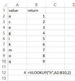
The formula in A12 is =VLOOKUP(“h”,A2:B10,2).

Vlookup will split the table in half and will look at the last value of the top half. If there is an uneven number of rows, it will grab the next row, too. So Vlookup will consider this range:

The table has 9 rows, so Vlookup looks at the fifth row of the data table.

With text values, “greater” and “smaller” refer to the position in an alphabetic sort. So “a” is smaller than “c” and “k” is greater than “c”.

The value “i” is greater than the search value “h”. Therefore, the desired value is above Excel row 6. Vlookup will then split this upper part of the table in half. Since there are 5 rows involved, the split will be done at the third row of the range:

Vlookup looks at Excel cell A4. This value “e” is smaller than the lookup value. That means that the value we want is not in the table range that was just inspectedd, so we can forget that part of the table. Next Vlookup looks at the lower half of the range from the previous step.

Again, the last value in that range is “i” and greater than the lookup value, so let’s split this range in half and look at the last row of the top half:

This range consists of one row only. There’s nothing more to split. The value is not an exact match, but the return column will be returned, anyway.

Vlookup with TRUE as the last parameter will deliver the value that is “equal to or smaller than” the lookup value.

Coming back to the example with the names at the top of the post:

The formula used is =VLOOKUP(“Akers”,B2:D5,2)

The range is split in half, the last value in the top half is greater than the lookup value, so the lower half of the table will not even be considered for further inspection. The top two rows will be split in half and a value smaller than “Carido” will be expected in the last cell of that next split. But the last value in a split has “Weiler” as the value. That is not smaller than the lookup value “Akers”. Hence an error is returned.

If we add one row to the lookup table range, the first pass of Vlookup will split the table of 5 rows in half, rounding up to contain the top three rows in the first pass. Now we use the formula

=VLOOKUP(“Akers”,B2:D6,2)

The value in cell B4 is a perfect match, so the value in column C is returned. Bingo! We have a correct result for an unsorted table, without the fourth parameter!

Magic? No, it is pure coincidence. Omitting the last Vlookup parameter on an unordered list MAY return the correct result, but the chances of that are rather slim.

In this case, it is pure luck that the lookup value matches the last entry of the range that Vlookup considers in this pass.

If you use Vlookup without the fourth parameter, you must ensure that the lookup table is sorted by the first column. Otherwise, any result you get back is as reliable as getting the lotto numbers from a toddler.

It may work, but in most cases it won’t.