Last week I saw some amazing Excel spreadsheets while I was attending the MVP Summit in Seattle and I thought I’d share some ideas. So here are step by step instructions on how to create a percentage chart with just the Excel grid and a sprinkle of conditional formatting. The goal we’re after looks like this:

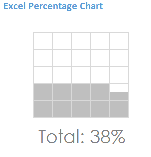
We’re looking at a grid of ten by ten cells that form a square (roughly). Each cell in this grid represents 1% of the whole. The number below the grid is represented visually by an according number of filled squares (or cells).

Here is how to do it:

Build the grid

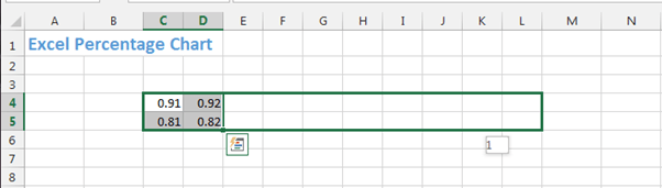
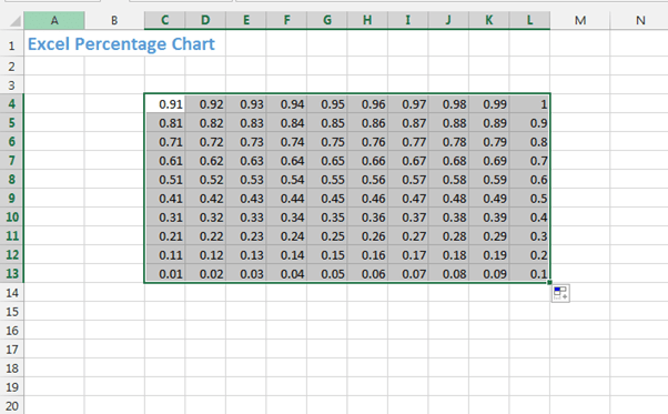
First we need the numbers from 0.01 to 1.00 in steps of 0.01 in a grid of 10 by ten cells. If you want, you can type these 100 numbers in manually, but there’s a faster way if you use the fill handle (the little dark square at the lower right corner of the active cell). We only need to type in four numbers. Let’s start in cell C4 and enter 0.91, then manually enter 0.92 in D4. Cells C5 and D5 will get the numbers 0.81 and 0.82 respectively.

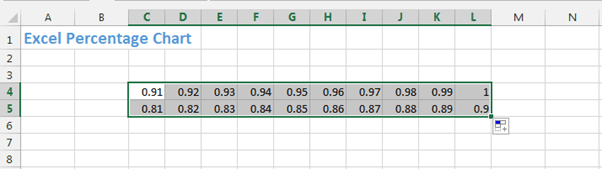
Select all four cells, then grab the lower right corner of cell D5 and drag it all the way across to cell L5.

Release the mouse button and you will see the numbers filled in and incremented accordingly:

Leave the cells selected, grab the fill handle in L5 and drag it down to row 13:

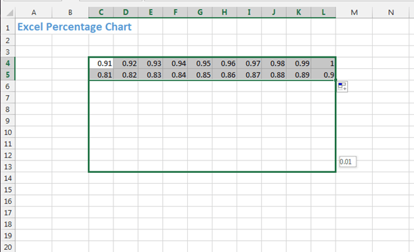
Release the mouse button and your 10 x 10 grid is filled with the correct numbers.

That was a bit faster than typing them all in, right?

Prepare the Total cell

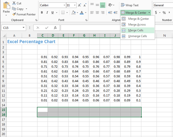
Leave one blank row below the grid, then select cells C15 to L16 and use the command Merge cells from the Alignment group of the Home ribbon.

After merging the cells, let’s enter a number, say 38% and do some number formatting. I’d like the cell to show the text “Total:” as well as the percentage number. Click the lower right corner of the Number group on the Home ribbon to open the Format Cell dialog. In the left hand pane select Custom at the bottom of the list. In the Type field enter the text
Total: 0%

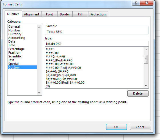
Note: The “” in front of the “:” sign is needed make sure it appears correctly. If we did not add this, Excel would get confused, since the “:” has a special use in time formats

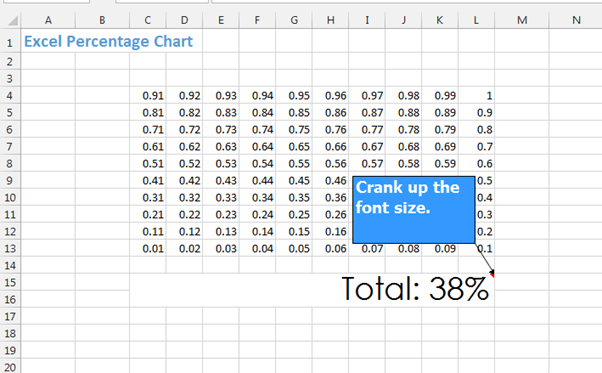
Hit OK and see how the cell shows text and number, even though the formula bar clearly shows that the cell only contains a number. Crank up the font size a bit. In this example I have used 28 pt Century Gothic.

Format the grid

Now we need to apply some TLC to the grid. Let’s hide the spreadsheet gridlines. On the View ribbon, untick the Gridlines box and the spreadsheet appears in uniform white.

The 10 x 10 grid should have light grey borders, so select the 100 cells …

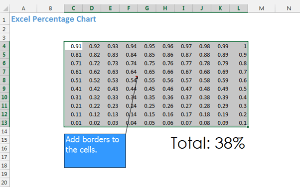
… and open the Format Cells dialog on the Border tab. Select a light grey colour from the colour drop-down and after that click the Inside and Outline boxes.

The cells now feature a faint grey grid, but the numbers are still showing. Here’s how to hide them for good: Keep the 100 cells selected, open the Format Cells dialog again and activate the Number tab. Choose the Custom option from the number categories and in the Type field enter three semicolons

;;;

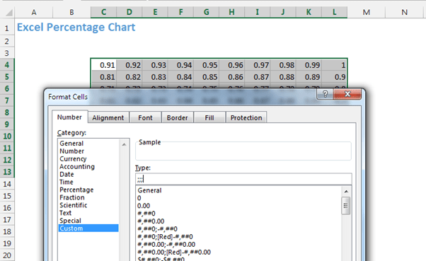
A number format in Excel consists of four parts to define positive, negative, zero and text values. The different parts are separated by semicolons. If the format definitions between the semicolons are missing, then the number will not be shown at all.

Now the grid is empty and we’ll set row height and column width to make it as close to square as possible:

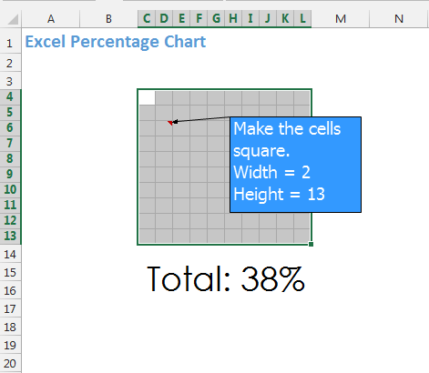
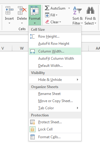
Select columns C to L and use the Format drop-down on the Home ribbon, where you will find the Width command. Then select rows 4 to 13 and use the same dropdown to select the Height.

Apply Conditional Formatting

The last step is the conditional formatting of the 100 cells. Again, this can be done in one go. Select the grid, then click the Conditional Formatting drop-down on the Home ribbon and select New Rule.

In the next dialog click Use a formula to determine which cells to format. In the formula box enter this formula:

=C4<=$C$15

Note the position of the $ signs. Only the $C$15 should have them. Don’t put them anywhere near C4.

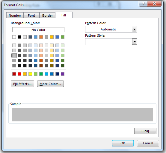
Click the Format button and select a darker grey as a fill colour.

Hit OK on all open dialogs.

That’s it. You’re done.

Change the number in the merged cell below the table and see the grid update with more or less grey blocks.

Of course, you can use other colours. Look at my Fruit Machine below. Click the blue cell and hit the Delete key to make the numbers change. Can you get all of them to display the same number?

Depending on your browser and/or screen resolution, you may see some of the grid lines wider than others. To download the workbook just click on the Excel icon in the dark bar below the spreadsheet.

Enjoy!

cheers, teylyn