Introduction
In the last part of this mini-series I’m showing how to draw attention to high and low values in Excel charts by using background fill. The first part of this mini-series showed how to present minimum and maximum values of a chart by simply sorting the data values in ascending or descending order. Part 2 looked at conditional formatting the columns themselves if they were the highest or lowest value in the chart. In Part 3, an image was used as a background fill on a stacked series.
Background fill
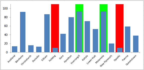
So let’s look at how to use a background fill for the highest and lowest data points. This can be achieved by plotting a column chart on the secondary axis. First, we need to prepare the data.
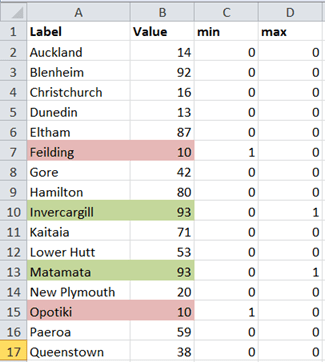
The minimum values are identified with
=IF(B2=MIN(Value),1,0)
The formula for the maximum values is
=IF(B2=MAX(Value),1,0)
The prepared data table looks like this:
Plot all three data columns as a clustered column chart. Then select the value series and send it to the secondary axis. Format the “min” and “max” series to have 100% overlap and a very small gap, like 10%.
Format the primary Y axis to a maximum of 1.
The tricky thing with this variant is to have the secondary Y axis appear on the left. To do this, follow these steps:
- On the Layout tab, select the Axes drop-down and show the secondary X axis. Now all the columns will be hanging upside down.
- Format the secondary X axis and let the vertical axis cross at category number 1
- Select the primary Y axis and format it to have no tick marks and no labels
- Format the secondary Y axis (which is now positioned at the left of the chart), and format it to let the Horizontal axis cross at axis value 0 (zero), which will put the columns on the base line again.
- Delete the primary X axis and fine tune the chart formatting as desired.
The result will look something like this:
Take your pick
I hope you have found this mini-series useful and will be able to apply the techniques to your charts.
The attached Excel workbook illustrates all charts above on separate sheets.
Enjoy.
